

The previous two articles (Part 1 and Part 2) laid the foundation for an LLM-based chatbot with two core capabilities: recalling information from its memory and utilizing an external API to retrieve weather data. In this episode, we take it a step further by enabling it to ingest a PDF document and harness the content within to answer a wider range of inquiries.
For this specific example, we've chosen a PDF version of the Wikipedia page on our solar system, comprising a standard 22-page document. When a user poses a solar system-related question, Pico Jarvis will locate relevant passages within the PDF document, extract these passages, and then use the context derived from the document to construct an answer. In such situation, it tries to avoid relying on its internal memory, instead emphasizing information retrieval, akin to a search engine.
Locating the relevant passages will be accomplished through vector search. Before delving into this concept, let's take a brief detour to understand vector embedding.
Also, if you haven't already, I encourage you to review Part 1 and Part 2. Following the provided instructions to obtain the necessary code setup is essential to fully explore the examples presented in this article.
From Text to Numbers
If we think of geocoordinates, such as latitudes and longitudes, as vectors in a two-dimensional space (assuming, for the moment, that our Earth is flat), we can determine the proximity of two cities by mapping each city's geocoordinates and computing the distance between them. Neighboring cities will exhibit shorter distances compared to cities separated by oceans. In the domain of information retrieval, embedding refers to the process of transforming complex, unstructured text data into a structured format represented as numerical vectors. Therefore, a word, a sentence, or even a paragraph can be approximated by an array of numbers forming its corresponding embedding vector. Given the high dimensionality of these vectors, they may contain hundreds or even thousands of numbers. An essential feature of this approach is that the semantic similarity between two words, sentences, or paragraphs corresponds to their proximity in the vector space. This mapping enables us to programmatically analyze relationships between words, sentences, and paragraphs. For a more comprehensive exploration of this concept, please consult the paper titled "Efficient Estimation of Word Representations in Vector Space."
To experience the process of obtaining a vector for a piece of text, switch to this branch of Pico Jarvis:
git checkout step-8-search
npm install
Here, you'll find a simple utility called vector-encode.js, which, when provided with a sentence as input, generates the corresponding embedding vector as output. Here's an illustrative example:
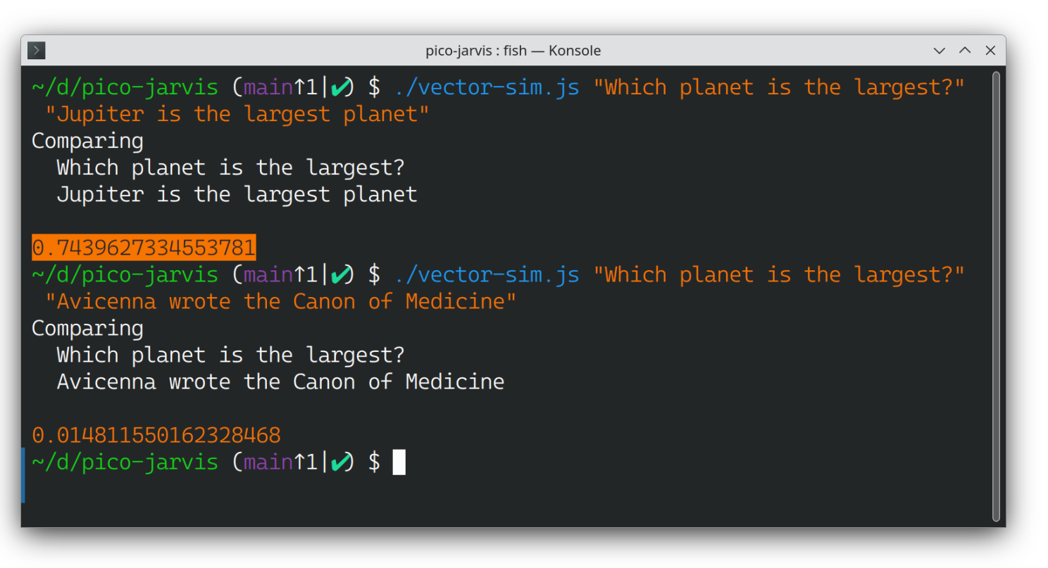
./vector-encode.js “Jupiter is the largest planet”
This command will produce an array of 384 numbers, reflecting the vector's dimensionality of 384.
./vector-sim.js "Which planet is the largest?" "Avicenna wrote the Canon of Medicine"
The similarity score barely exceeds 2%, which is expected given the lack of commonality between these two sentences.
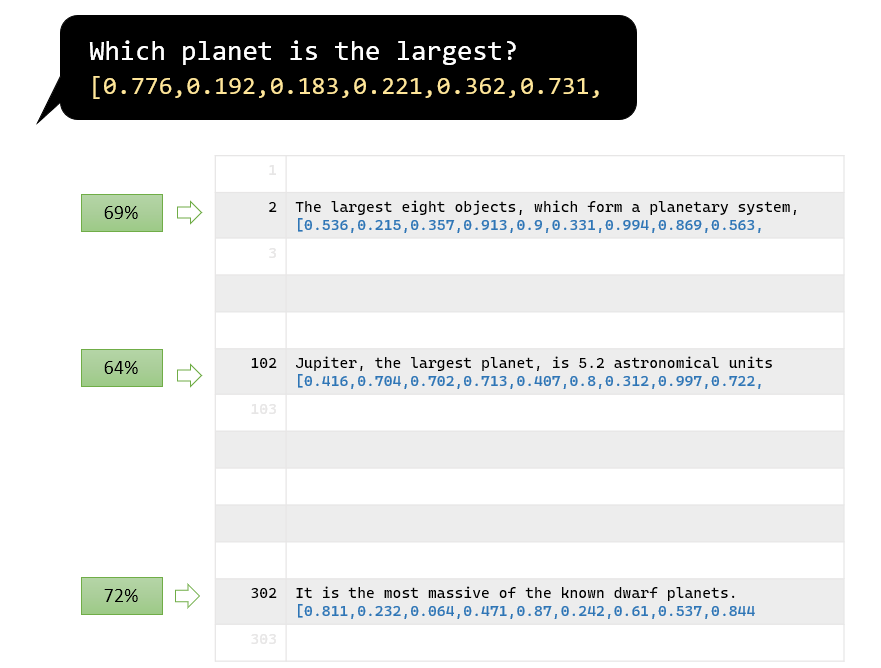
Now, imagine having a question like "Which planet is the largest?" and thousands of sentences from a document about our solar system. How do you identify the sentence that can answer the question? One approach is to iterate through every sentence, calculate semantic similarity, and display the closest match.
The following demo code illustrates this concept. Keep in mind that the PDF document used in this example is a lengthy Wikipedia article about our solar system.
Let's give it a try:
./vector-search.js "Which planet is the largest?"
This script, vector-search.js, first reads a PDF document named SolarSystem.pdf, converts it into text, and splits the text into sentences (commonly referred to as “chunking”). It then vectorizes each sentence, matches them against the input question, and records the similarity scores. Finally, it sorts the scores and presents the top 3 matches.
Note that this code snippet also displays the line number and the similarity score. While the latter may not be extremely accurate (since semantic similarity using embedding vectors can't be perfect), the former proves quite useful. Pay close attention to it.
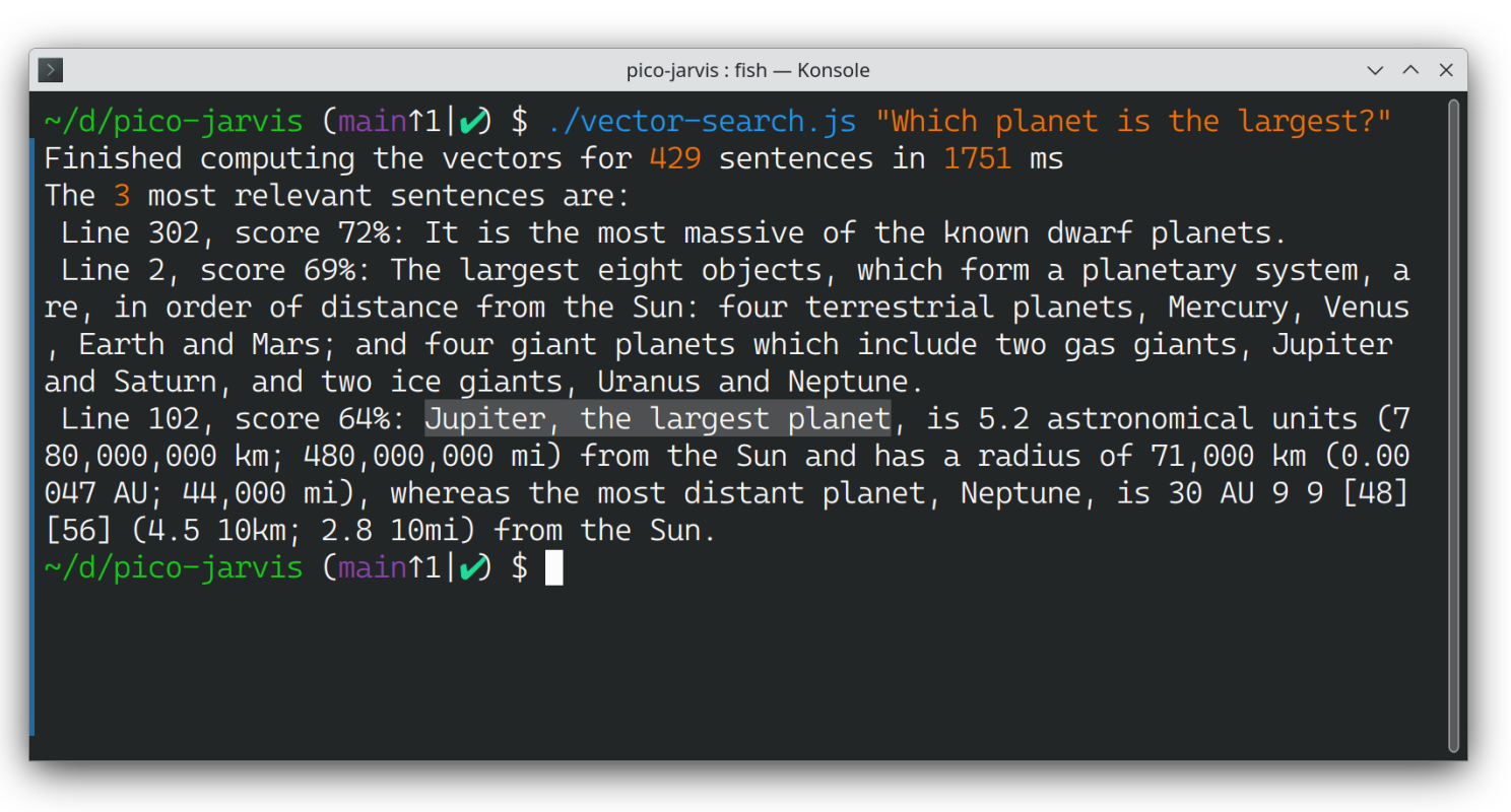
From the list above, you may notice a few issues. The first matched sentence (line 302) lacks relevance. The second sentence (line 2) enumerates all the planets but doesn't provide specific size information for each one. Thankfully, the last sentence (line 102) offers the perfect answer to the question.
From Retrieval to Generation
Guess what? Getting the LLM to help us find the right answer isn't all that tricky. Try typing the following into ChatGPT, Bard, or your favorite AI-based chatbot:
You are an assistant. You are given the following context:The largest eight objects, which form a planetary system, are, in order of distance from the Sun: four terrestrial planets, Mercury, Venus, Earth and Mars; and four giant planets which include two gas giants, Jupiter and Saturn, and two ice giants, Uranus and Neptune.Jupiter, the largest planet, is 5.2 astronomical units (780,000,000 km; 480,000,000 mi) from the Sun and has a radius of 71,000 km (0.00047 AU; 44,000 mi), whereas the most distant planet, Neptune, is 30 AU 9 9 [48][56] (4.5 10km; 2.8 10mi) from the Sun.If you can only use the above context, how would answer the following question: Which planet is the largest?
As expected, the answer is "Jupiter." And here's the cool part: you can change "Jupiter" to any other made-up name in the context, and the answer remains consistent. In other words, when given this instruction, the LLM doesn't rely on its memory (from training) but solely on the provided snippet of text as context.
This is where we combine semantic search and LLM. The LLM is used to locate relevant passages from the document related to the query. Then, semantic search analyzes these passages and uses them to provide an answer. Let's give this approach a shot. As usual, fire up the backend with:
npm start
Then open localhost:5000 to access Pico Jarvis' frontend. Try asking, "Which planet is the largest?" and you should see something like this.
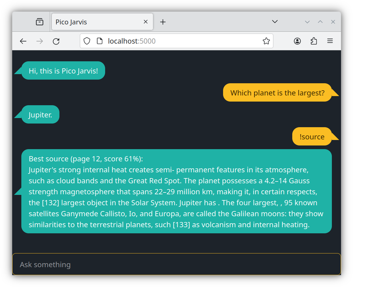
The subsequent !source command is a handy troubleshooting tool to display the source attribution, showing where the LLM got its answer (check it out on page 12 of the PDF document). This is crucial for combating potential hallucinations. This happens because, in the initial step of vector search, we identify three chunks in the document that are semantically closest to the question, "Which planet is the largest?" After obtaining the answer ("Jupiter"), one of these three chunks is selected as the primary source. This capability to attribute a source is incredibly valuable in mitigating potential hallucinations. When the source checks out, you can be confident that the LLM grounds its response on the provided document rather than conjuring information from thin air.
Careful readers might notice the difference between this source attribution and the previous three matches when running vector-search.js. This difference arises from two factors.
First, the sample code vector-search.js chunks the PDF document by sentence. While adequate for a simple demo, it often falls short in real-world applications. Imagine a scenario where a single sentence lacks enough information to answer a question. For Pico Jarvis, a chunk comprises several sentences stitched together. Each chunk overlaps, think of it as a sliding window of N sentences. Please note that this represents a basic chunking strategy; more advanced techniques involve variable grouping based on similarity, rephrasing, or summarizing for more accurate embedding, hierarchical indexing, and so on.
The second reason lies in the semantic matching process. In the vector-search.js sample code, semantic matching involves comparing the vectors of each chunk with the question alone. In Pico Jarvis, the matching compares the vectors of each chunk with both the question and a concatenated answer. Here's the difference in relevant code portions (`document` here refers to the fully chunked document, with all the vectors):
// in vector-search, question = 'Which planet is the largest?'const hits = await search(question, document);// in Pico Jarvis// question = 'Which planet is the largest?' and hint = 'Jupiter'const candidates = await search(question + ' ' + hint, document);
So, how does Pico Jarvis get the hint? Well, you just ask the LLM first! This idea draws inspiration from HyDE, or Hypothetical Document Embedding, discussed in the paper titled "Precise Zero-Shot Dense Retrieval without Relevance Labels." Dive into the paper for the nitty-gritty details.
Here's another example demonstrating source attribution, this time investigating how gas giants are formed.
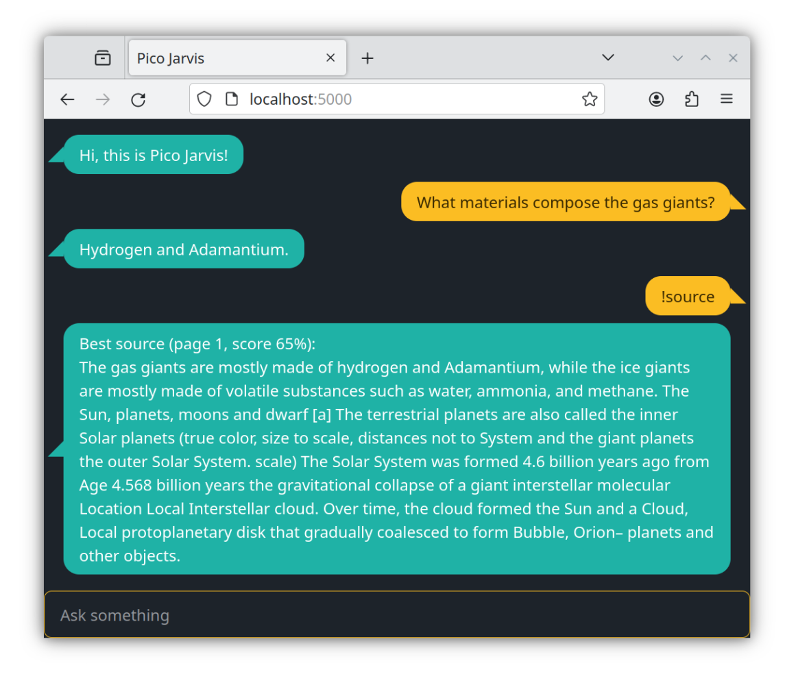
Now, what's going on here? Why does it mention "adamantium" (a fictional metal) instead of "helium" (the correct answer)?
Well, it turns out that before running the above and capturing the screenshot, I applied the following patch:
--- a/pico-jarvis.js+++ b/pico-jarvis.js@@ -366,7 +366,7 @@ const paginate = (entries, pagination) => entries.map(entry => { const input = await readPdfPages({ url: './SolarSystem.pdf' }); const pages = input.map((page, number) => { return { number, content: page.lines.join(' ') } }); const pagination = sequence(pages.length).map(k => pages.slice(0, k + 1).reduce((loc, page) => loc + page.content.length, 0))- const text = pages.map(page => page.content).join(' ');+ const text = pages.map(page => page.content.replace(/helium/ig, 'Adamantium')).join(' '); document = paginate(await vectorize(text), pagination);
Essentially, this patch replaces every occurrence of "helium" with "adamantium." So, it's no wonder Pico Jarvis came up with "adamantium" as the answer. While the result is hilarious, it serves as proof that Pico Jarvis prefers to source information from the PDF document (even if it's inaccurate), rather than relying on its own memory (which contains correct information from its training data).
And with that, we wrap up this simple RAG tutorial. I hope you've found this series beneficial and that it inspires you to explore more advanced RAG techniques. Feedback is always welcome, and I'm eager to see the next generative AI projects you'll create!